Kmeans From Scratch With Numpy And Pandas

Hello Everyone! It’s a cool -2F here in the windy city. I grabbed my coffee and set out to build the KMeans Clustering algorithm from scratch using NumPy and Pandas.

As a refresher KMeans is an unsupervised clustering algorithm. The general methodology goes as follows:

1. Define the number of target clusters.
2. Randomly select cluster centers from the data pool.
3. Do 1-Nearest Neighbor to classify all the other points to defined centers.
4. Average those points classified together to redefine the new cluster center points.
5. Repeat 3-4 a reasonable amount of times

Alright, let us get into the details.

Start by doing your imports. In this notebook I will be using the plot.scatter functionality of Pandas which runs matplotlib under the hood, so we will drop in the inline display tweak for jupyter notebooks.

import numpy as np
import pandas as pd
from matplotlib import pyplot as plt
%matplotlib inline

Function Definitions

make_blob: Used to create randomly generated floats of data to give the exercise a basic foundation of clusters. r1 and r2 are the bounds, d is the dimensionality (we’re doing 2 dimensions), and p is the number of points we want.

def make_blob(r1,r2,d,p):
    return [(r2-r1)*np.random.random_sample((d,))+r1 for i in range(p)]

initialize_KMeans_Centers: When starting out we do not have cluster centers defined. The methodology calls for randomly selecting cluster centers. We will pass in our dataframe of points and c is the number of clusters we’re defining. Using NumPy’s random.choice function we select c number of items between 0 and len(df) which represents our range in the dataframe. We then reindex centers as a stanalone dataframe and set the class column to it’s index. It makes a good unique identifier.

def initialize_KMeans_Centers(df, c):
    centers = df.iloc[np.random.choice(len(df),c,False)].copy()
    centers.reset_index(inplace=True, drop=True)
    centers['class'] = centers.index
    return centers

nearest: This function is essentially the kNN algorithm but it only retrieves the 1-Nearest item’s classification. Each point p in our dataframe will go through and determine which of the cluster centers c it is closest to and retrieve that classification.

def nearest(p,c):
    point = p['pt1':'pt2']
    clsf = sorted([[np.linalg.norm(point-item[1]['pt1':'pt2']),item[1]['class']] for item in c.iterrows()])[0][1]
    return clsf

classify: This function is what calls the nearest function across all the data points in the dataframe using Pandas’ apply method and a lambda expression to apply our nearest function to our dataframe points.

def classify(df,ctrs):
    df['class'] = df.apply(lambda x: nearest(x,ctrs),axis=1)
    return df

new_centers: This performs very similar functionality as initialize_KMeans_Centers except that this step happens in the subsequent looping part of the algorithm when we are averaging clusters that were classified together to determine new cluster centers. Pandas’ groupby allows us to group by the classifications we have assigned and returns the mean for the pt1 and pt2 columns in the dataframe giving us new cluster centers.

def new_centers(df):
    centers = df.groupby('class').mean()
    centers.reset_index(inplace=True, drop=True)
    centers['class'] = centers.index
    return centers

Initialize KMeans

Alright, that was the hard part. Now let us setup the example. Here we are defining that we want to find 3 clusters. For simplicy and ease of visualization we are using 2 dimensions (x and y), but these dimensions will be based on your real world data which can extend hundereds of dimensions. npts is the number points we will generate per blob, and in this example I am making 3 blobs because I’m seeking 3 clusters. Again, this is just random data for demonstration purposes. Finally, cycles defines how many times I want to re-average the clusters and re-classify the points. You would adjust this number based on your time, resource, and accuracy constraints and needs.

clusters = 3
dims = 2
npts = 30
np_pts = make_blob(30,100,dims,npts) + make_blob(20,80,dims,npts) + make_blob(40,60,dims,npts)
cycles = 5

Here we take our random data which was created in NumPy and convert it into a dataframe dfpts. We will also create a class column that will act as a placeholder for our future classification activity.

dfpts = pd.DataFrame(np_pts,columns=['pt1','pt2'])
dfpts['class'] = 0

We initialize our first pass center points by randomly selecting from our dataframe using the initialize_KMeans_Centers function call. This will be the only time we use this function.

centers = initialize_KMeans_Centers(dfpts, clusters)
centers

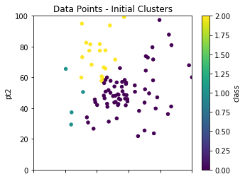
Using the classify function we previously defined we pass in our data frame of points and the cluster centers and classify will attach a classification to each of our data points. If you review the function above you will see this is done via the Panda’s apply and lambda approach and calling nearest on each data point.

dfpts = classify(dfpts,centers)

Plot the Initial Pass

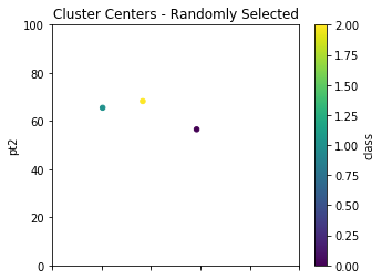
Ok, great, so we have now initialized everything up to providing the data points their first classification. Let us look at some visuals so we can see what is going on. We will use Panda’s plot.scatter on the randomly selected cluster centers centers.plot.scatter and also on our data points dfpts.plot.scatter.

init_centers = centers.copy()
init_centers.plot.scatter(x='pt1',y='pt2',c='class',\
                     colormap='viridis',figsize=(5,4),\
                     xlim=(0,100),ylim=(0,100),title="Cluster Centers - Randomly Selected");

init_pts = dfpts.copy()
init_pts.plot.scatter(x='pt1',y='pt2',c='class',\
                     colormap='viridis',figsize=(5,4),\
                     xlim=(0,100),ylim=(0,100),title="Data Points - Initial Clusters");

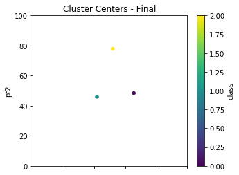
Iterating to Final Clusters

As previously mentioned, we randomly select our initial starting points to cluster on, but the results are not final until we take multiple passes to achieve a more robust clustering solution. We had previously defined in our setup cycles as 5. This loop calls new_centers and classify over and over to re-average and re-classify our clusters. With real world data, something you may want to try is storing the results of the cluster centers over the iterations and finding the point at which the change in those averages becomes negligible.

for times in range(cycles):
    centers = new_centers(dfpts)
    dfpts = classify(dfpts,centers)
    

centers.plot.scatter(x='pt1',y='pt2',c='class',\
                     colormap='viridis',figsize=(5,4),\
                     xlim=(0,100),ylim=(0,100),title="Cluster Centers - Final");

dfpts.plot.scatter(x='pt1',y='pt2',c='class',\
                     colormap='viridis',figsize=(5,4),\
                     xlim=(0,100),ylim=(0,100),title="Data Points - Final");

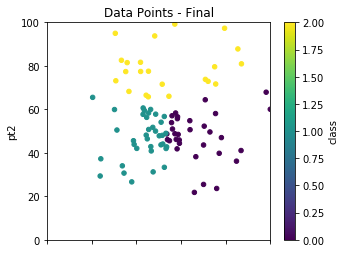
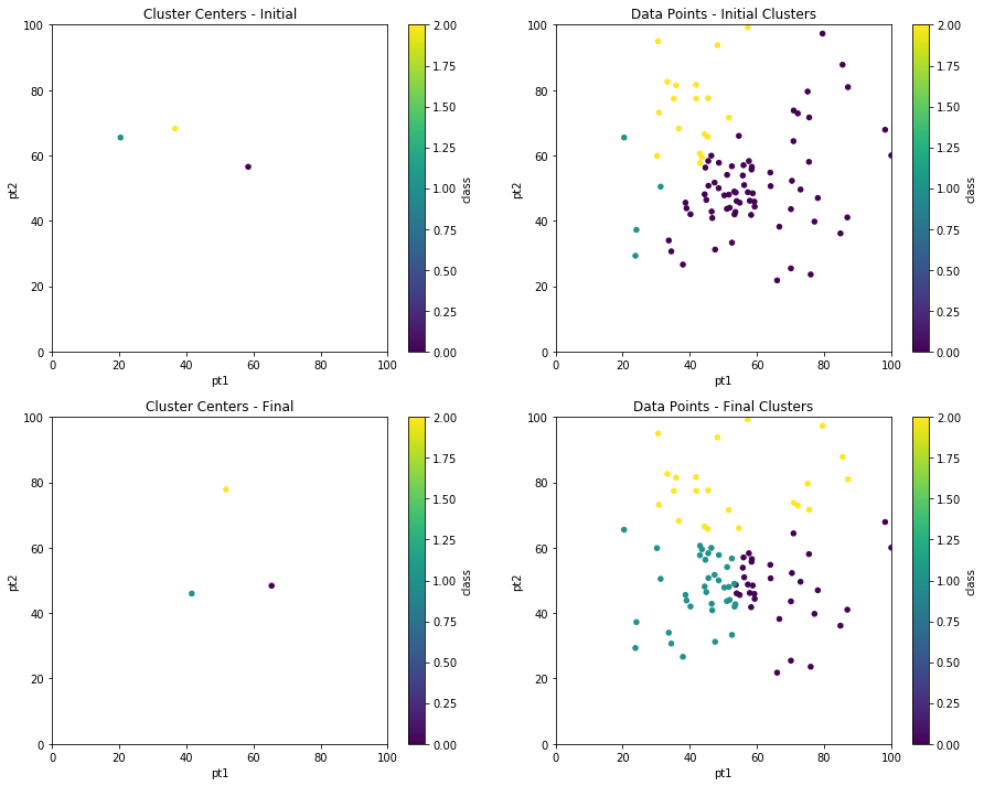
Finally, we can compare the before and after cluster centers and data point clustering using subplots.

fig, axes = plt.subplots(nrows=2, ncols=2,figsize=(15,12))
init_centers.plot.scatter(x='pt1', y='pt2', c='class', colormap='viridis',\
                     xlim=(0,100),ylim=(0,100),title="Cluster Centers - Initial",ax=axes[0,0]);
init_pts.plot.scatter(x='pt1', y='pt2', c='class', colormap='viridis',\
                     xlim=(0,100),ylim=(0,100),title="Data Points - Initial Clusters",ax=axes[0,1]);
centers.plot.scatter(x='pt1', y='pt2', c='class', colormap='viridis',\
                     xlim=(0,100),ylim=(0,100),title="Cluster Centers - Final",ax=axes[1,0]);
dfpts.plot.scatter(x='pt1', y='pt2', c='class', colormap='viridis',\
                     xlim=(0,100),ylim=(0,100),title="Data Points - Final Clusters",ax=axes[1,1]);

You should know I initially set out to do this without Pandas. I quickly realized there was huge benefit in using Pandas to achieve this. I hope you enjoyed this exercise. And please reach out with any questions or feedback. Thanks for reading, and remember:

Stay Chaotic – Stay Neutral

ARI

K Nearest Neighbors From Scratch

Happy New Year! It’s going to be an awesome 2019. I can feel it!

We start out the new year with a challenge I had been discussing with some colleagues:

Let’s build KNN from scratch without using SkLearn or any pre-built libraries.

A debate ensued as to whether numpy would be allowed, but in the end I decided I would have three methods of doing this: vanilla, numpy, and scipy. Additionally, I am a fan of one-liners. I know, I know, they can get pretty long and un-pythonic. But I think they are fun, so I do them anyway. In the end we have 6 ways of doing KNN. Using the three previously mentioned approaches both as one-liners and non-one-liners.

Setup

We will use numpy to initialize the list of points that we will find the nearest neighbors for. That is not to say we are cheating as we are only setting up some random state. In the real world the ‘neighbors’ can come in many formats and here we are simply initializing.

We also import scipy for the ‘euclidean’ approach to this solution.

The ‘kn’ variable determines how many nearest neighbors we are looking for, while ‘npts’ is how many points we have on our list to check against.

The ‘dims’ variable is how many dimensions we want our points to be, again, this will be determined by your real data, but here we allow to test for data among any number of dimensions.

While I create the random data using numpy I actually need two versions of the data for the numpy and non-numpy methods. This is why there is a np_pts / pts and np_newpt / newpt. It’s the same data, just cast as a numpy array and a list.

import numpy as np
from scipy.spatial.distance import euclidean
kn = 3
npts = 100
dims = 10
np_pts = [np.random.randint(1,100,dims) for i in range(npts)]
pts = [list(pt) for pt in np_pts]
np_newpt = np.random.randint(1,100,dims)
newpt = list(np_newpt)
print("New Point as a Numpy Array:",np_newpt)
print("New Point as a List:",newpt)

New Point as a Numpy Array: [39  6 68 48 14 76 57  5  8 55]
New Point as a List: [39, 6, 68, 48, 14, 76, 57, 5, 8, 55]

Now that our points and new point are initialized let us build out KNN using vanilla, numpy, and scipy.
You will notice the pattern will repeat itself using the three methods. The steps are:

• Iterate though the points
• Calculate the distance
• Append the resulting distance and the data point to a distances list
• Sort the newly formed list of distances
• Show only the top n based on our ‘kn’ variable via list slicing

Specifically when calculating the distance via the vanilla method, we need to take the extra step of resetting the sums_of_squares for each point we are iterating through, summing up those squared distances in the second for loop, and taking it’s square root.

Vanilla Python

distances = []
for pt in pts:
    sums_of_squares = 0 
    for i,j in zip(newpt,pt):
        sums_of_squares += (i-j)**2
    dist = sums_of_squares**0.5
    distances.append([dist, pt])
print(kn,"Nearest Neighbors - Vanilla:")
[print(i) for i in sorted(distances)[:kn]];
    

3 Nearest Neighbors - Vanilla:
[76.50490180374065, [30, 28, 87, 24, 38, 63, 82, 13, 62, 56]]
[78.8098978555359, [25, 20, 18, 76, 35, 76, 45, 6, 18, 98]]
[79.58643100428615, [52, 20, 22, 79, 6, 52, 30, 30, 21, 82]]

Using Numpy

distances = []
for pt in pts:
    dist = np.linalg.norm(np_newpt-pt)
    distances.append([dist, pt])
print(kn,"Nearest Neighbors - Numpy:")
[print(i) for i in sorted(distances)[:kn]];

3 Nearest Neighbors - Numpy:
[76.50490180374065, [30, 28, 87, 24, 38, 63, 82, 13, 62, 56]]
[78.8098978555359, [25, 20, 18, 76, 35, 76, 45, 6, 18, 98]]
[79.58643100428615, [52, 20, 22, 79, 6, 52, 30, 30, 21, 82]]

Using Scipy

distances = []
for pt in pts:
    dist = euclidean(newpt,pt)
    distances.append([dist, pt])
print(kn,"Nearest Neighbors - Scipy:")
[print(i) for i in sorted(distances)[:kn]];

3 Nearest Neighbors - Scipy:
[76.50490180374065, [30, 28, 87, 24, 38, 63, 82, 13, 62, 56]]
[78.8098978555359, [25, 20, 18, 76, 35, 76, 45, 6, 18, 98]]
[79.58643100428615, [52, 20, 22, 79, 6, 52, 30, 30, 21, 82]]

One-Liners

As previously mentioned, I’m a fan of one-liners. So having performed the exercise of building KNN from scratch using the approaches above, we can take these for loops and convert them into list comprehensions.

Vanilla Python

vanilla_one_liner = sorted([[sum([(i-j)**2 for i, j in zip(newpt,pt)])**0.5, pt] for pt in pts])[:kn]
print(kn,"Nearest Neighbors - Vanilla One-Liner:")
[print(i) for i in vanilla_one_liner];

3 Nearest Neighbors - Vanilla One-Liner:
[76.50490180374065, [30, 28, 87, 24, 38, 63, 82, 13, 62, 56]]
[78.8098978555359, [25, 20, 18, 76, 35, 76, 45, 6, 18, 98]]
[79.58643100428615, [52, 20, 22, 79, 6, 52, 30, 30, 21, 82]]

Using Numpy

numpy_one_liner = sorted([[np.linalg.norm(np_newpt-pt), pt] for pt in np_pts])[:kn]
print(kn,"Nearest Neighbors - Numpy One-Liner:")
[print(i) for i in numpy_one_liner];

3 Nearest Neighbors - Numpy One-Liner:
[76.50490180374065, array([30, 28, 87, 24, 38, 63, 82, 13, 62, 56])]
[78.8098978555359, array([25, 20, 18, 76, 35, 76, 45,  6, 18, 98])]
[79.58643100428615, array([52, 20, 22, 79,  6, 52, 30, 30, 21, 82])]

Using Scipy

scipy_one_liner = sorted([[euclidean(newpt,pt), pt] for pt in pts])[:kn]
print(kn,"Nearest Neighbors - Scipy One-Liner:")
[print(i) for i in scipy_one_liner];

3 Nearest Neighbors - Scipy One-Liner:
[76.50490180374065, [30, 28, 87, 24, 38, 63, 82, 13, 62, 56]]
[78.8098978555359, [25, 20, 18, 76, 35, 76, 45, 6, 18, 98]]
[79.58643100428615, [52, 20, 22, 79, 6, 52, 30, 30, 21, 82]]

I really enjoyed this exercise. I hope you all enjoyed breaking outside of the canned packaged libraries and getting your hands a little dirty. Thanks for reading, and remember:

Stay Chaotic – Stay Neutral

ARI